This week’s blog post is more geared toward housekeeping and fortifying my model. My reasoning for this is because my forecast has tumbled downhill in the past three weeks. When I began to incorporate more district-specific variables into my district forecast, I ran into the issue of working with data limited in scope (like expert predictions, turnout data, and advertising numbers).
The reality in which my model was operating contained few observations per district (oftentimes 2-3 observations), which is not ideal when searching for trends. The more observations, the better and more precise the observation can be. One limitation of this is that not all districts have had the same shape and voters since 1960 (where my data goes back to). However, districts do not change all too much, so I will still continue to use districts going back decades, because we are working with extremely limitated data. Also, much of this district-specific data was not collected for each district. Therefore, I was not only making imprecise predictions but also I was making predictions for a small subset of districts (not all districts, which is my goal).
Therefore, going forward, I believe the best variables to employ are those that are collected far back into history and are available for almost all districts. Hopefully, this will allow me to make better predictions for each district in the country.
Shocks in an Election
This week I explored data related to shocks in election cycles. A shock in an election cycle is an event that is seen as groundbreaking and unexpected, with the potential of solely changing the outcome of the election. Examples would include natural disasters, political scandals, etc. Another commmon term for a shock is “October Surprise,” which, as the name suggests, is an election-altering event that happens in October, right before the election.
Scholars Achen and Bartels stated with supporting data that voters tend to irrationaly take out their anger and place blame on incumbent elected officials at the ballot box after a shock has occurred, whether or not the incumbent truly bears responsibility for the event or response. They used an example of a beach town’s incumbent officials difficulty getting re-elected after shark attacks — something officials virtually have no control over.
However, shocks may not be as important as one may believe. Schoalr Andrew Healy instead claims that voters tend to punish incumbents for an ineffective response or having no response at all, not directly for the happening of the event. I believe this to be the correct interpretation of how shocks affect elections, and Marco Mendoza Aviña goes even further, describing how COVID-19 did not cpst Trump the 2020 election.
Therefore, I will bypass using shocks as a variable for elections. It is not entirely clear how big of an effect they have over voters, and if there is an effect, how long it lasts. I believe my time is better served by fortifying my model with variables that I know work well through previous research and experimentation.
Pooled Models
A pooled model is a good idea for when you have districts with less data available than others. This is a concept that employs a strategy of “borrowing” data from districts with similar variables. In retrospect, employing a pooled model for my previous weeks would be interesting, since almost 350 districts were left without observations and thus predictions.
However, I do not believe a pooled model to be the most efficient forecast for my model. My first reasoning is that, even if I were to be able to borrow data from similar districts based off demographic data, for example, I would still be basing predictions off 2-3 observations on average. This is not an efficient way to find trends and narrow down confidence intervals. My second reason for this is that I have found my national-level variables to be better predictors than the district specific ones. Thus, borrowing data is unnecessary, as national-level data is available to be applied to all districts.
So without the need to employ a pooled model, I will begin fortifying my model with national-level variables to forecast the national and district-level elections.
Incumbency Variable
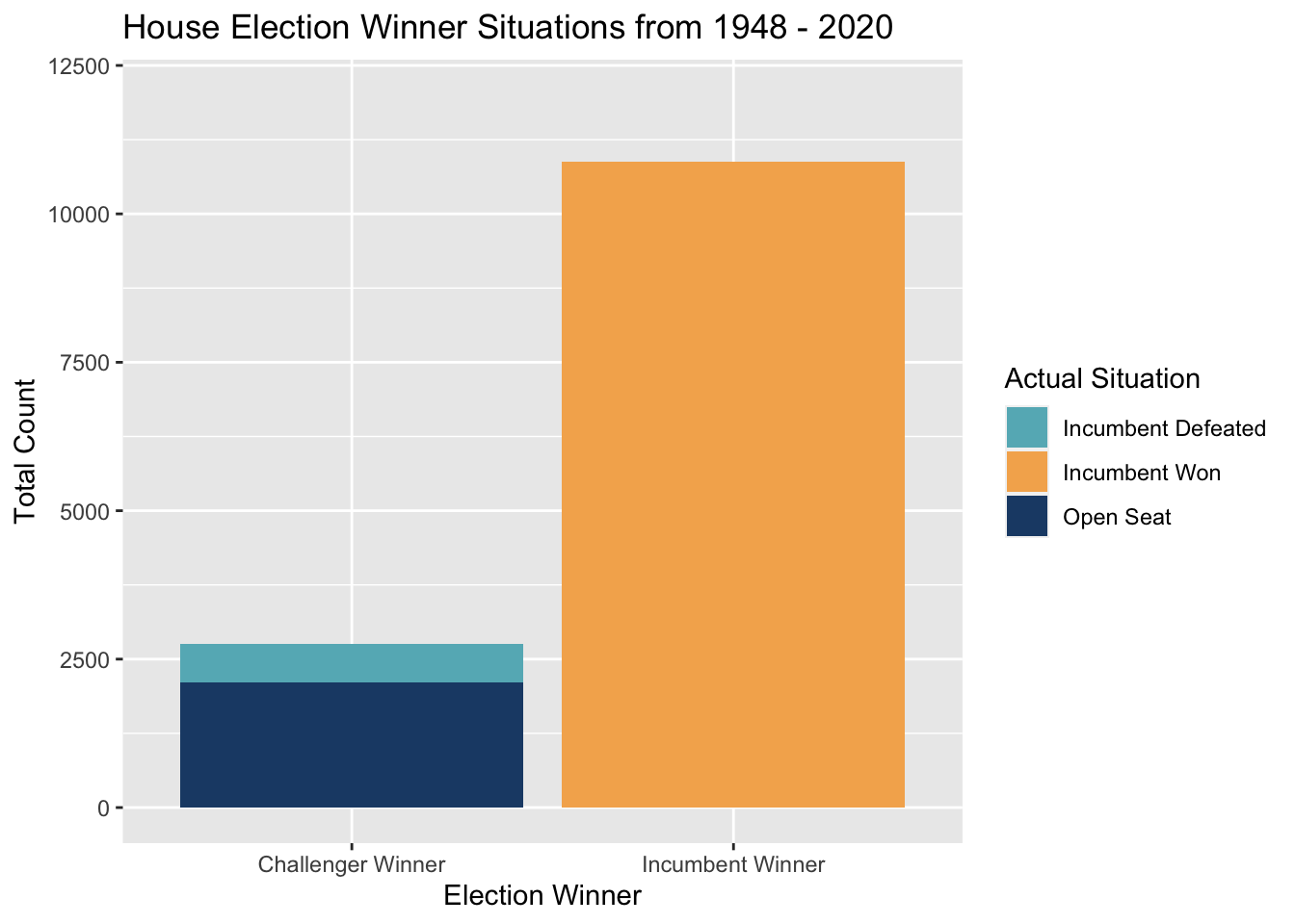
Professor Ryan Enos has described to his Gov 1347 class at Harvard how incumbents, statistically, win way more than their challengers. It’s no secret that elected officials tend to stay in Congress for a long time. Below, I look at just how often these incumbents win re-election, and the results in the plot and corresponding table with numbers are stark.
The biggest takeaway from historical data on incumbency is how challengers beat incumbents essentially 4.7% of the time. Incumbents, on the other hand, can decide their fate a little over 85% of the time, by either running and handily winning or by retiring due to old age or the knowledge that they might be defeated in the upcoming election. Thus, if an incumbent runs, it is probably a great sign that they see a clear path to winning. This is a variable I will seek to include into my model.
Presidential Approval Variable
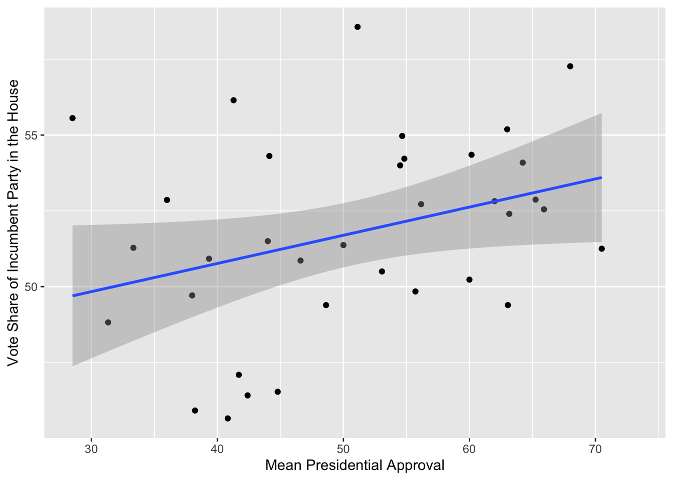
Presidential approval is another variable that is widely looked at as one that possesses predictive value. Steve Kornacki visited our Gov 1347 class and stated how this variable is one of his few that he believes to be highly important as he predicts the midterms. Since midterm elections often are framed as referendums and checks on the president and his party, I will look to see how the incumbent party in the House fares. By the looks of it, it could foster some predictive value. Therefore, I will experiment with this in my model too.
National Model
Now, I will begin building out my model as I forecast my district-by-district prediction. The variables I will look to experiment with are (and form some kind of combination):
- Percent change in Real Disposable Income (RDI) Change from April to November of an election year
- The aggregate democratic margin in the generic congressional ballot polls up to 50 days before an election
- Mean presidential approval number from August to November of an election year
- Whether an incumbent is running for re-election or not
| Model 1 | Model 2 | Model 3 | Model 4 | |
|---|---|---|---|---|
| (Intercept) | 52.00 *** | 52.00 *** | 52.00 *** | 52.00 *** |
| (0.59) | (0.31) | (0.31) | (0.32) | |
| rdi_change_pct | -0.35 | -0.15 | -0.02 | -0.02 |
| (0.60) | (0.32) | (0.35) | (0.35) | |
| natl_genericpoll_mean_dem_margin | 2.70 *** | 2.88 *** | 2.88 *** | |
| (0.32) | (0.37) | (0.37) | ||
| incumb_running_count | 0.38 | 0.44 | ||
| (0.39) | (0.41) | |||
| mean_pres_approval_num | 0.18 | |||
| (0.35) | ||||
| N | 29 | 29 | 29 | 29 |
| R2 | 0.01 | 0.74 | 0.75 | 0.75 |
| All continuous predictors are mean-centered and scaled by 1 standard deviation. *** p < 0.001; ** p < 0.01; * p < 0.05. | ||||
The biggest takeaway from these model outputs is just how predictive the national generic ballot democratic polling margin is. With a p-value consistently < 0.001, I am convinced the variable in its format must be included. When I look to other variables, I am left with a troubling reality where none of the others seem to bolster my forecast. In the background, I tested combining each variables with the national generic ballot democratic polling margin variable, and pairing the RDI percent change variable with it provides a model with the smallest predictive intervals and an adjusted r-squared still right at the level of the other pairings. Below, I will show my predictions using these two variables in my models.
District by District Predictions
Here I have built a GLM-based district-by-district model that also includes incumbency variables on top of the national generic ballot democratic polling margin and RDI change percent variables. It has eliminated the phenomenon where I predicted vote shares below 0% and above 100% (which I experienced in previous weeks).
While this is a step in the right direction, my predictions and predictive intervals highlight some more problems: my intervals are way too wide and predicted democratic vote shares all seem to hover around 47% (+/- a few percentage points). With only 4 districts boasting a democratic vote share above 50%, this model is unrealistic (while becoming better at the same time). A house majority of 431-4 for Republicans is nowhere close to what will or ever has happened for a party. Thus, I need to narrow down my intervals, so I can arrive at more accurate predictions. This may require me to actually utilize district-specific variables and somehow extrapolate the data to any missing districts and years so that I can continue having a large number of observations per district for a more precise interval and predicted value.
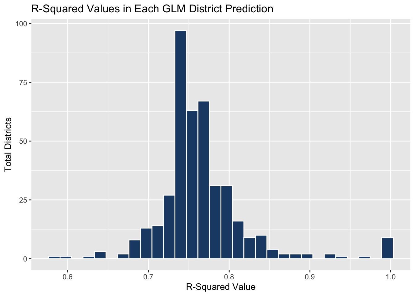
I have also included an R-squared histogram that shows vast improvement in this model over previous weeks’. This improvement is shown through the consistently high R-squared values, which is a good sign since last week each district boasted an R-squared of 1, which is dangerous in research and especially when predicting values dependent on multiple combinations of unknown variables like election modeling.
R-Squared Values by District
Notes:
This blog is part of a series of articles meant to progressively understand how election data can be used to predict future outcomes. I will add to this site on a weekly basis under the direction of Professor Ryan D. Enos. In the run-up to the midterm elections on November 8, 2022, I will draw on all I have learned regarding what best forecasts election results, and I will predict the outcome of the NE-02 U.S. Congressional Election.