In this blog, I will seek to highlight how incumbency and expert ratings can be used in predicting elections. To start, I will compare how expert predictions compare to the actual election results in 2018, and then extrapolate the variable of expert ratings into my election modeling forecast
Seatshare from 2018 Congressional Elections by Party and Incumbency
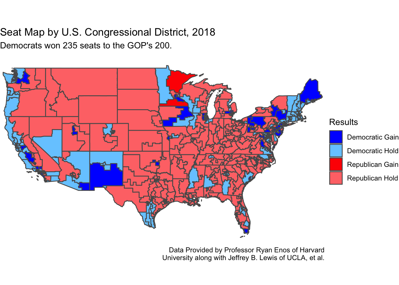
Below, I have mapped the actual result of the 2018 congresisonal midterms in terms of seat share attained by each party. Additionally, I have included the districts in which an incumbent party lost their seat to the other party. In total, the Democrats flipped 46 seats from the previous Congress, and Republicans flipped only 5, indicating just how successful Democrats were in 2018. I will elaborate more on incumbency later, especially because of how only 34 incumbents ran and lost in the 2018 election cycle (4 lost in their primary elections, and 30 lost in the general election). Incumbency alone does not seem to be a factor per Adam R. Brown. However, the advantages that go along with incumbency tend to provide incumbents an edge over their opponent.
Expert Predictions
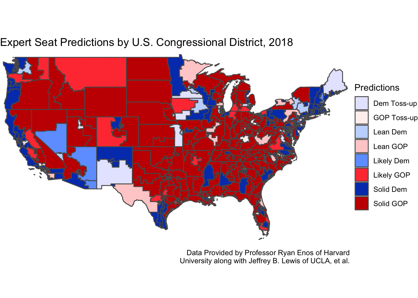
The map below displays the seat share predicted by the “experts” in the 2018 cycle. These predictions hinge on a variety of factors, culminating into their overall district “rating” that provides a probability of the favored party’s chances at winning, as detailed by Nate Silver of FiveThirtyEight. The categories “toss-up, lean, likely, and solid” go in order of increasing probability to win, respectively, with a toss-up signifying a race that is close to 50/50. We can see how the frequency of “Toss-up” or districts with a slight lean are uncommon, to say the least. This displays just how noncompetitive most races typically are. The effects of this lack of competition are substantial when it comes to predicting elections: most noncompetitive districts lack accurate polling and interest, therefore decreasing predictors that can be utilized in models.
To counteract a lack of information about a specific district, expert outlets will often lean on the fundamental predictors (economy, incumbency, and demographics) that are not affected by a campaign and generic ballot congressional polls, or they will look to borrow available, accurate polling from districts with a large amount of similarities. This is how entire predictions maps, like the one below, are created. And one last note, it is best practice to average these expert predictions (from historically successful and trusted outlets like FiveThirtyEight, Cook Political Report, etc.), like we do with national polls, as to account and offset for any bias in the predictions (ideally).
Accuracy of Expert Predictions
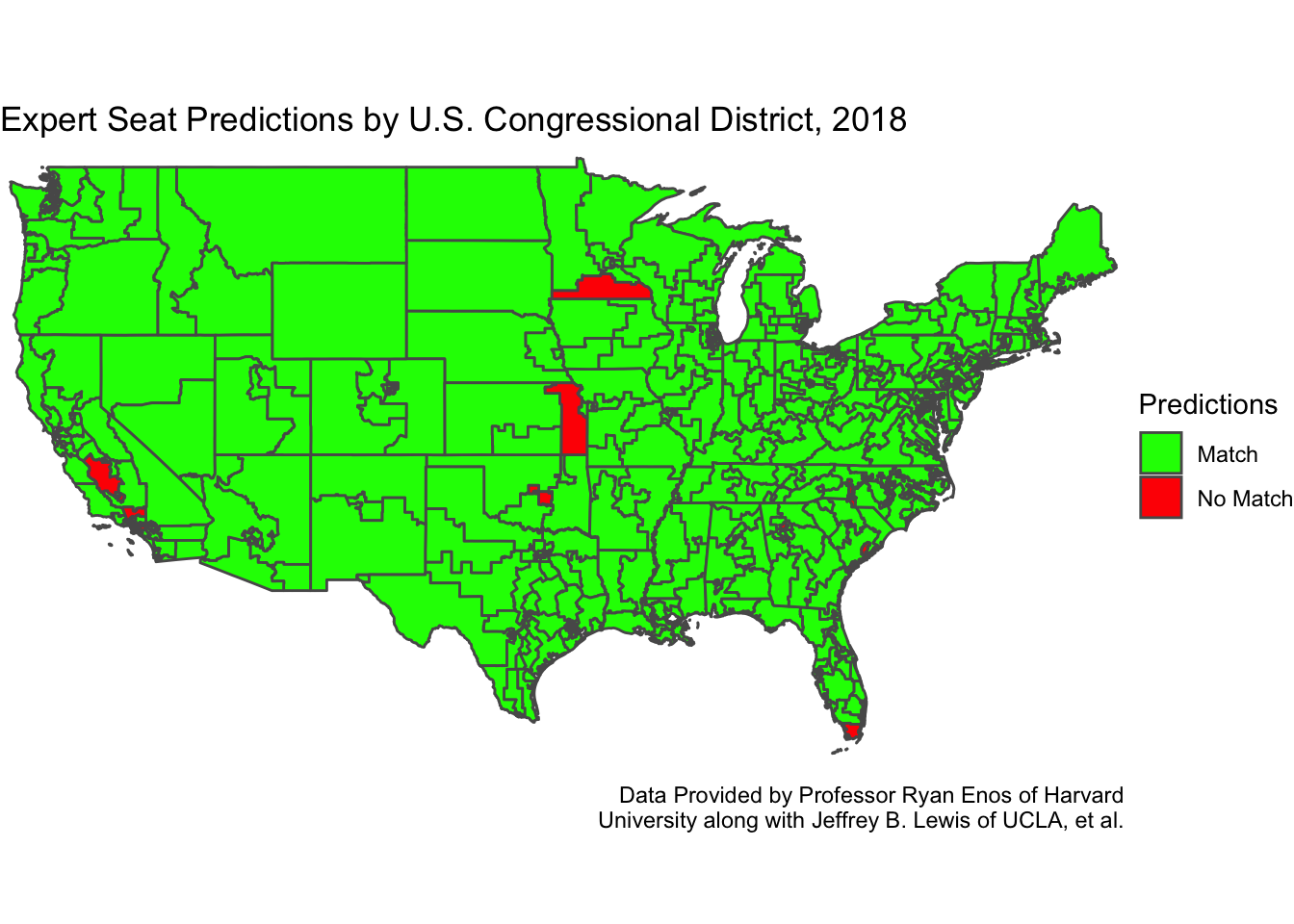
Like weather predictions by expert meteorologists, expert election predictions are not always correct. Often, it is advantageous to see just how accurate the predictions are and where the mistakes lie, so one can hopefully make adjustments in the future. Below, the accuracy of the expert predictions for 2018 are plotted, displaying that the experts almost predicted all districts correctly.
Incumbency Advantage and Expert Predictions
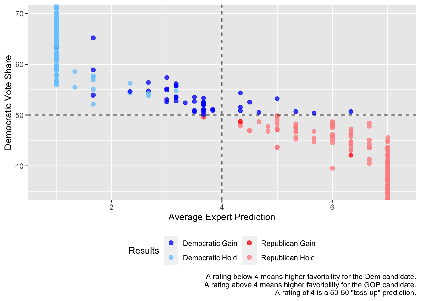
The US map and graph of the experts’ accuracy are testaments to the reliability in using their predictions for elections. By many measures, the average of their ratings tend to produce incredibly accurate results. One aspect to notice is that if a Democrat was predicted to win in 2018, they almost always won, while many Republican candidates who were favored to win ultimately lost. Inaccurate predictions lie in quadrants 1 and 3. This could indicate a potential bias that neglected the Democratic party’s strength in 2018.
Another evident aspect to the plot is seeing how many incumbents ran and lost in the election. Ultimately, 34 incumbents who ran for re-election lost, with 4 losing their primary election and 30 losing their general election. Out of 374 races where an incumbent ran for reelection, only 34 losing is stark look at their resiliency. In fact, it has been noted that incumbents who seek reelection tend to win more than 90% of the time.Even though some incumbents who have held office for a long time could be set at a disadvantage, this variable of incumbency seems to be an efficient predictor of elections.
Incumbency seems to be a priviledged advantage for those in a race. However, it has been documented that incumbency alone (meaning other structural advantages are held constant) is not enough to sway voters. The advantage lies in the incumbent’s opportunity to gain name recognition and association with accomplishments, to raise huge sums of money as someone in power, the already-built-up wall that discourages challenges to challenge someone who seemingly has a 90% chance of winning, and the fact that incumbents may simply be more politically competent as they have already been through the campaign gauntlet.
Updated Prediction Model
Because expert ratings incorporate incumbency into their predictions alongside other fundamental and polling variables, I will look to incorporate these into my forecasting model. Below I have listed my predictions for the Democratic Party’s vote share by district (where expert predictions are currently available from the dataset I was provided through my class).
Results by Congressional District
##             state district       pred
## 1          Alaska       AL  69.441391
## 2         Arizona        1  45.280269
## 3         Arizona        2  48.271210
## 4         Arizona        6  51.159434
## 5      California       21  40.961311
## 6      California       22  78.507143
## 7      California       25  57.050825
## 8      California       26  55.987778
## 9      California        3  47.469831
## 10     California       45  54.579310
## 11     California       47  40.660737
## 12     California       49  49.730952
## 13     California        9  51.162657
## 14       Colorado        3  56.083159
## 15       Colorado        7  39.849298
## 16    Connecticut        4  44.472978
## 17    Connecticut        5  53.678653
## 18        Florida       13  38.614971
## 19        Florida       15  56.684286
## 20        Florida       16  81.334853
## 21        Florida        2  79.821954
## 22        Florida       22  47.398042
## 23        Florida       27  53.281050
## 24        Florida        7  49.221475
## 25        Georgia       12  50.649111
## 26        Georgia        6  53.246089
## 27       Illinois       11  48.755840
## 28       Illinois       13  50.269034
## 29       Illinois       14  53.164321
## 30       Illinois       17  50.171631
## 31       Illinois        6  54.795918
## 32       Illinois        8  63.235380
## 33           Iowa        1  47.235039
## 34           Iowa        2  45.149679
## 35           Iowa        3  48.469607
## 36         Kansas        3  51.077168
## 37          Maine        2  46.704484
## 38       Maryland        6  54.998532
## 39       Michigan       11  57.148761
## 40       Michigan        3  37.346297
## 41       Michigan        7  48.262001
## 42       Michigan        8  50.261327
## 43      Minnesota        1  49.843152
## 44      Minnesota        2  42.591603
## 45      Minnesota        3  52.851374
## 46      Minnesota        8  48.605832
## 47       Missouri        2  51.043785
## 48       Nebraska        2  47.033199
## 49         Nevada        3  48.980095
## 50         Nevada        4  49.719551
## 51  New Hampshire        1  45.980325
## 52  New Hampshire        2  50.933172
## 53     New Jersey       11  56.461111
## 54     New Jersey        2  51.234360
## 55     New Jersey        3  48.386586
## 56     New Jersey        5  42.081903
## 57     New Jersey        7  53.896826
## 58     New Mexico        1  43.124130
## 59     New Mexico        2  54.259972
## 60       New York        1  49.092371
## 61       New York       11  45.858288
## 62       New York       18  48.493028
## 63       New York       19  49.501115
## 64       New York        2  51.631034
## 65       New York       22  48.861609
## 66       New York       25 -47.075003
## 67       New York        3  44.548958
## 68       New York        4  46.624566
## 69 North Carolina       13  56.387236
## 70 North Carolina        6  52.841280
## 71 North Carolina        7  49.945113
## 72 North Carolina        9  54.313462
## 73           Ohio        1  87.190455
## 74           Ohio       10   5.826923
## 75           Ohio       13  38.233198
## 76           Ohio       15  34.708216
## 77           Ohio        7  20.450256
## 78         Oregon        5  42.982183
## 79   Pennsylvania        1  55.479730
## 80   Pennsylvania       10  34.685212
## 81   Pennsylvania       12  50.645417
## 82   Pennsylvania       17 199.390820
## 83   Pennsylvania        6  49.804774
## 84   Pennsylvania        7  49.070487
## 85   Pennsylvania        8  48.940465
## 86 South Carolina        1  52.377619
## 87          Texas       23  48.443030
## 88       Virginia       10  49.144492
## 89       Virginia        2  48.179994
## 90       Virginia        5  48.671982
## 91       Virginia        7  54.493396
## 92     Washington        3  48.595811
## 93     Washington        8  53.187348
## 94      Wisconsin        3  41.034989
Here we can see some predictions that are plausible, especially when compared to previous election data. This includes my particular district of interest in this blog, Nebraska’s 2nd congressional district, where the Democratic candidate is projected to earn 47.03% of the vote. This falls in line with previous elections in the district, since the Democratic candidate has often fallen just short of winning (and barely winning in 2014).
However, there are some serious pitfalls to this model that need more examining.
The first pitfall is some resulting Democratic Party vote share numbers. The Democrat in NY-25 is predicted to earn -47.08% of the vote, and a candidate never can win a negative share of the vote. Also, the candidate in PA-17 is projected to earn 199.39% of the vote, and a candidate can never win greater than a 100% share of the vote.
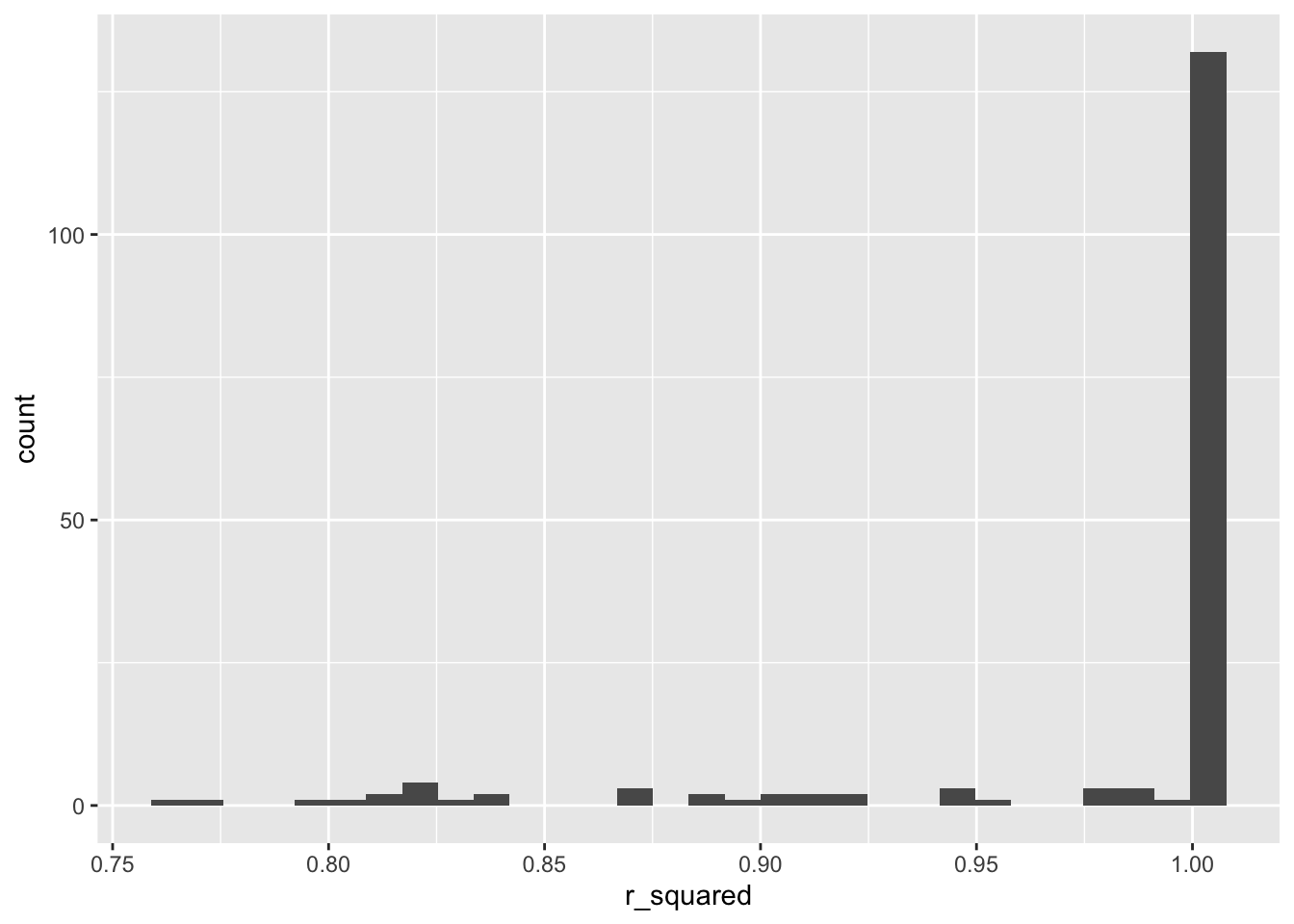
Second, the R-squared numbers for my predictions by district are graphed below. While a higher R-squared is always desired, a value of 1 often should raise eyebrows in suspicion. Due to the sheer number that boast an R-squared value of 1, I am very pessimistic of this model and its effectiveness.
R-Squared Comparisons
Thus, after some smooth sailing, this blog has shown that my model has taken a step back in its path toward improvement and accuracy. I suspect that the pitfalls of this model are the result of some coding errors and mistakes on the set-up of my model. Hopefully, next week will set me back on my course.
Notes:
This blog is part of a series of articles meant to progressively understand how election data can be used to predict future outcomes. I will add to this site on a weekly basis under the direction of Professor Ryan D. Enos. In the run-up to the midterm elections on November 8, 2022, I will draw on all I have learned regarding what best forecasts election results, and I will predict the outcome of the NE-02 U.S. Congressional Election.